Results 

The objective of this study was to determine the relationship between monthly sea ice concentrations and diatom species assemblages. This relationship is crucial in understanding the significance of diatom assemblages in downcore ocean sediments in Baffin Bay, Davis Strait and Labrador Sea. The results of this study are based on three multivariate statistical techniques; 1) Hierarchical Cluster Analysis; 2) Multiple Regression Tree (MRT) Analysis; 3) Direct gradient analysis using non-linear multidimensional scaling (NMDS). These techniques were chosen because in general they are used to determine the relationship between predictor variables (sea ice concentration) and response variables (diatom species). 

1. Cluster Analysis 

To determine whether there is a difference in diatom assemblages among stations, a ward hierarchical cluster analysis using bray-curtis distance matrix was performed. Based on the primary split it appears that the lower latitude stations (2, 10 and 6) are closely related, while the higher latitude stations (28, 32, 40, 36, 55, 24, and 47) are related. The further splits accounts for differences among locations, likely in terms of proximity to coast, changes in salinity and sea surface temperature.

Figure 11. Dendrogram from a ward hierarchical cluster analysis of sampling stations based on diatom species abundance. The initial split separates the high latitude sampling sites from the lower latitude sampling sites.

2. Multiple Regression Tree Analysis 

 A Multiple Regression Tree (MRT) analysis was performed to determine the relationship between monthly sea ice concentrations and diatom species in each station (Figure 12; Table 3). MRT allows one to determine the size of the tree (the number of nodes) based on the variance explained. The results of the MRT suggested that February sea ice concentration is the most significant predictor variable, accounting for 32% of variance (Table 3). Sea ice is generally at the maximum concentration and extent between February and March. From the primary split, we can infer that there are two diatom assemblages based on whether there is a high (>68.2%) February sea ice concentration, or lower February sea ice concentration (<68.2%). Therefore we have now have two distinct diatom assemblages. The MRT also shows that there are only 2 of the stations contain this low February sea ice concentration diatom assemblage, while the remaining 9 stations are characterized by the high February sea ice concentration diatom assemblage. It it likely that the 2 stations are in fact the lower latitude stations, which may be characterized as a transitional area between temperate and arctic oceanic conditions. To determine whether there may be two more groups of diatom assemblages, I chose to produce an MRT analysis with two splits. The second split in the regression tree is based on September sea ice concentrations.Sea ice is generally at the minimum annual concentration and extent in September. We can infer that there are now two more diatom assemblages, one in which sea ice completely disappears during summer (<0.63%) and one when sea ice is present throughout the entire summer (>0.63%). A summary of the diatom assemblages based on the MRT analysis is given in Table 4.

Figure 12. Regression tree created from MRT analysis.  The diatom species are separated into 4 assemblages, 1. present in low February sea ice, 2. present in high February sea ice, 3. present when September sea ice exists, 4. present when there is no September sea ice. Data used for the MRT analysis was standardized.

Table 3. Variance explained by each split on the tree given by MRT analysis. 

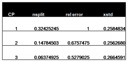
Table 4. Diatom assemblages based on MRT analysis. Four diatom assemblages were determined using the MRT analysis: 1) <68% February sea ice concentration; 2) >68% February sea ice concentration; 3) <0.6% September sea ice concentration and; 4) >0.6% September sea ice concentration.

3. Direct Gradient Analysis using NMDS

A direct gradient analysis using Nonlinear Multidimensional Scaling (NMDS) was used to determine the cause and effect relationship between the predictor variables (sea ice concentration) and the response variables (diatom species; figure 13). The direct gradient analysis was carried out to gain more specific details on the relationshp between the species and the sea ice concentration data. Also, to determine the results relative to the sampling stations. The resulting plot of the analysis shows station ID numbers (circled numbers), species abundance (blue vectors) and monthly sea ice concentrations (red vectors). Each variable is plotted based on its relationship with other variables. For example, stations that are close together have a close relationship, while those that are far apart are not closely related. Similarly, the position of the vectors signifies a relationship. For example, August sea ice is closely related to species A, B, I, J and K, meaning where there is high august sea ice, there is high abundances of these species.

Figure 13. Analysis produced by the non-linear multidimensional scaling technique. Circled numbers indicate the station numbers, letters represent diatom species and months represent monthly sea ice concentrations. 

The results of the gradient analysis using NMDS show a relationship between high August, September and October sea ice concentrations and the species A (Fossula arctica), B (Fragilariopsis cylindrus), I (Porosira glacialis) and J (Nitzschia grunowii). The species F (T. Hyalina) is between the August, September and October vectors and the February vector. This can be interpreted as the species F. hyalina being equally related to these months. These results agree with the results of the MRT analysis, where all five of the aforementioned species are associated with high February sea ice concentrations and high September sea ice concentrations.

Conclusions
Based on preliminary analysis using previous research to classify diatom species environmental niches, two distinct assemblages were observed; one consisting of over 50% sea ice diatoms, while the other consisting of less than 50% sea ice species. The sea ice diatom assemblage decreased in relative abundance with a decrease in latitude. Planktonic and brackish water diatom species were shown to replace the sea ice species in lower latitudes.

The results of the cluster analysis show the separation of the higher latitude stations and the lower latitude stations with respect to diatom species present. According to the MRT analysis, February sea ice concentration may be the most important environmental variable, accounting for most of the variance in the diatom species. The diatom species associated with high (>68%) February sea ice include Fossula arctica, Fragilariopsis cylindrus, Thalassiosira antarctica var. borealis, Thalassiosira hyalina, Porosira glacialis and Nitzschia grunowii. The direct gradient analysis using NMDS agreed that this species assemblage is associated with high sea ice in all four months considered in the study. In previous studies in the North Atlantic, five species have been associated with the Marginal Ice Zone (MIZ) assemblage.

The results of this study will enable me to continue to work on the down core analysis of diatom assemblages in the study area.